Ensure your y- and x-axis are Grattan style guide-consistent and doesn't hang off the edge of the chart.

These functions also hide the '0' label when the axis starts at 0.

grattan_y_continuous(
  expand_bottom = 0,
  expand_top = 0.015,
  expand = NULL,
  labels = grattan_label_hide_zero,
  ...
)

scale_y_continuous_grattan(
  expand_bottom = 0,
  expand_top = 0.015,
  expand = NULL,
  labels = grattan_label_hide_zero,
  ...
)

grattan_x_continuous(
  expand_left = 0,
  expand_right = 0.015,
  expand = NULL,
  labels = grattan_label_hide_zero,
  ...
)

scale_x_continuous_grattan(
  expand_left = 0,
  expand_right = 0.015,
  expand = NULL,
  labels = grattan_label_hide_zero,
  ...
)

Arguments

expand_bottom

default is 0. This will ensure that your x-axis is at the bottom value of your plotted data. Increase to add some buffer between the lowest point in your data and the x-axis. Note that the value is interpreted as a fraction of the total plotting space - a value of 1 will add white space equal to the whole area of your data.

expand_top

default is 0.015. This will ensure that a small amount of white space is added to the top of your chart. Increase to add more white space.

expand

a vector of expansion constants, as you would pass to `scale_y_continuous()` or `scale_x_continuous()`, typically created with `ggplot2::expansion()`. Defaults to NULL, in which case the expansion is set by `expand_bottom` and `expand_top` (or `expand_left` and `expand_right`). If you supply `expand`, those arguments are ignored.

labels

labels for the axis breaks, passed to `scale_y_continuous()` or `scale_x_continuous()`. The default uses comma formatting and hides the '0' label when the axis starts at 0. Supplying your own labels (such as `scales::label_percent()`) replaces this, so the '0' label will be shown.

...

other arguments passed to `scale_y_continuous()` or `scale_x_continuous()`, such as `limits` and `breaks`.

expand_left

default is 0. This will ensure your y-axis is at the lowest value of your plotted value.

expand_right

default is 0.015. This will ensure that a small amount of white space is added to the right of your chart.

Examples

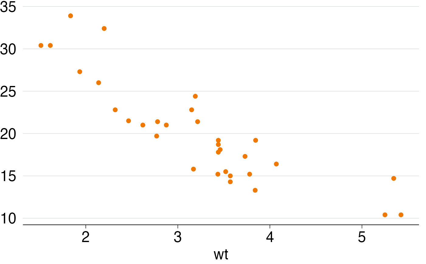
# Here's a basic chart in the Grattan style:
library(ggplot2)

p <- ggplot(mtcars, aes(x = wt, y = mpg)) +
    geom_point() +
    theme_grattan()
p


# In the example above, the top label on the y-axis is hanging off the top.
# To fix:

p <- ggplot(mtcars, aes(x = wt, y = mpg)) +
     geom_point() +
     grattan_y_continuous() +
     theme_grattan()

p


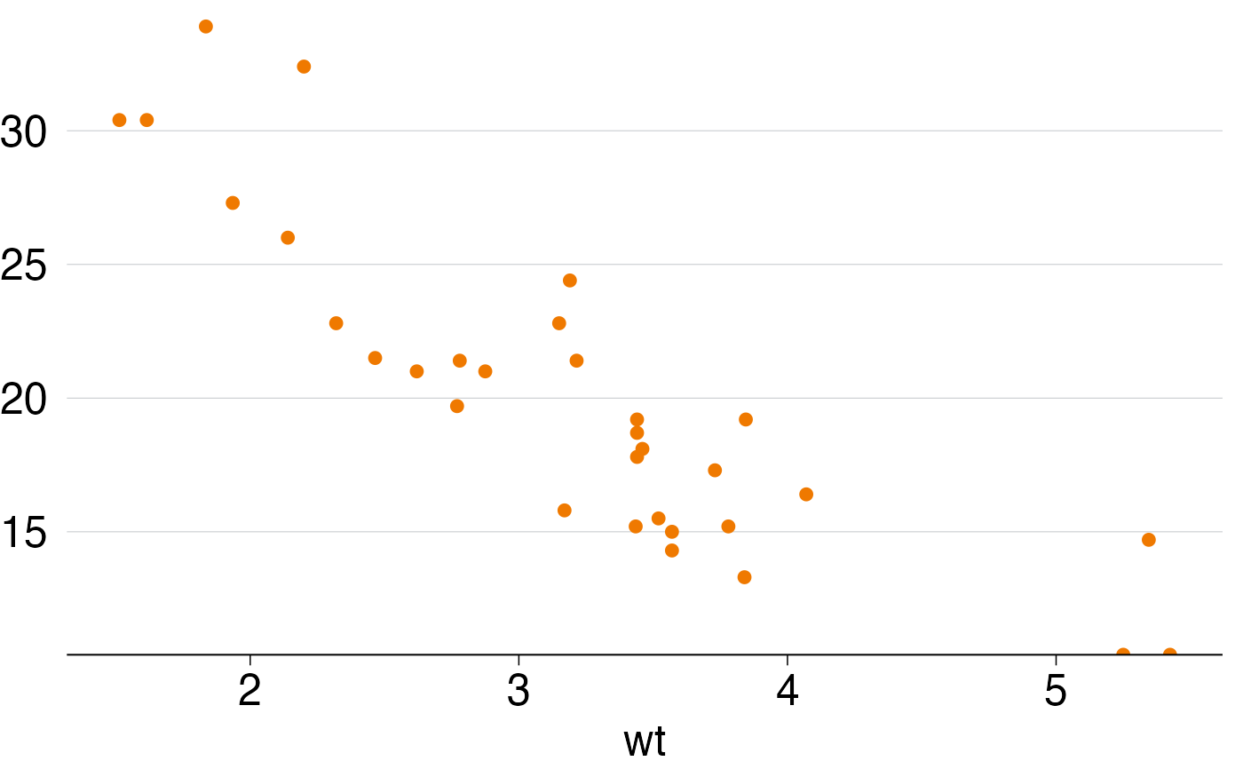
# Now the top of the chart looks fine, but the bottom has two points
# (at the lower right) that are partially obscured.
# We could fix this by doing:

p <- ggplot(mtcars, aes(x = wt, y = mpg)) +
     geom_point() +
     grattan_y_continuous(expand_bottom = 0.015) +
     theme_grattan()

p


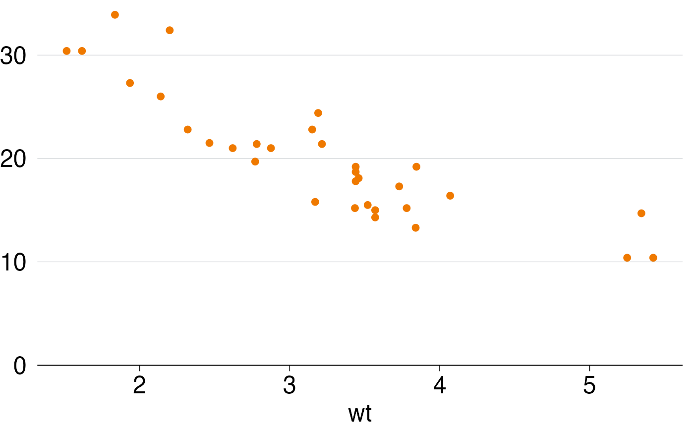
# Alternatively, set the limits of the chart (in this example we'll set
# the lower limit to 0, but you could use some other value
# like 10 in this case).Note that by setting the second value of limits
# to NA, we're telling ggplot2 to calculate the upper limit as usual based
# on the data. All the usual arguments of `scale_y_continuous()`
# (limits, breaks, labels, etc.) can be used.

p <- ggplot(mtcars, aes(x = wt, y = mpg)) +
     geom_point() +
     grattan_y_continuous(limits = c(0, NA)) +
     theme_grattan()

p