Using grattantheme

This vignette explains how to use grattantheme to quickly and consistently apply Grattan chart formatting to charts made in R using ggplot.

When creating a chart using ggplot we have to:

Choose a dataset;
Map variables to chart aesthetics aes();
Choose a geom_.

For example, using the in-built iris dataset:

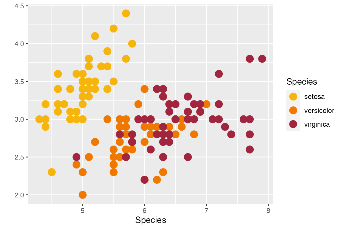
plot <- ggplot(iris,
               aes(x = Sepal.Length,
                   y = Sepal.Width,
                   colour = Species)) +
        geom_point(size = 4) +
        labs(x = "Species",
             y = "",
             colour = "Species")

This successfully plots the data we want to plot:

But it doesn’t yet look like a Grattan chart. To adjust the look we adjust ‘theme’ elements, like axis.ticks.x = element_line(colour = "black") to adjust the axis tickmarks on the x axis; panel.grid.major.x = element_blank() to turn off vertical gridlines; and so on; and on; and on. We also need to adjust aesthetic colours to the Grattan palette; setting, for example, fill = "#F68B33". The grattantheme package contains tools and shortcuts to simplify this process.

Formatting theme elements with `theme_grattan()`

The function theme_grattan() contains all of the Grattan theme adjustments in one handy command. Combined with grattan_colour_manual, which easily changes colours of aesthetics, your R chart will be ready for a report or a slide in no time.

plot + 
  theme_grattan()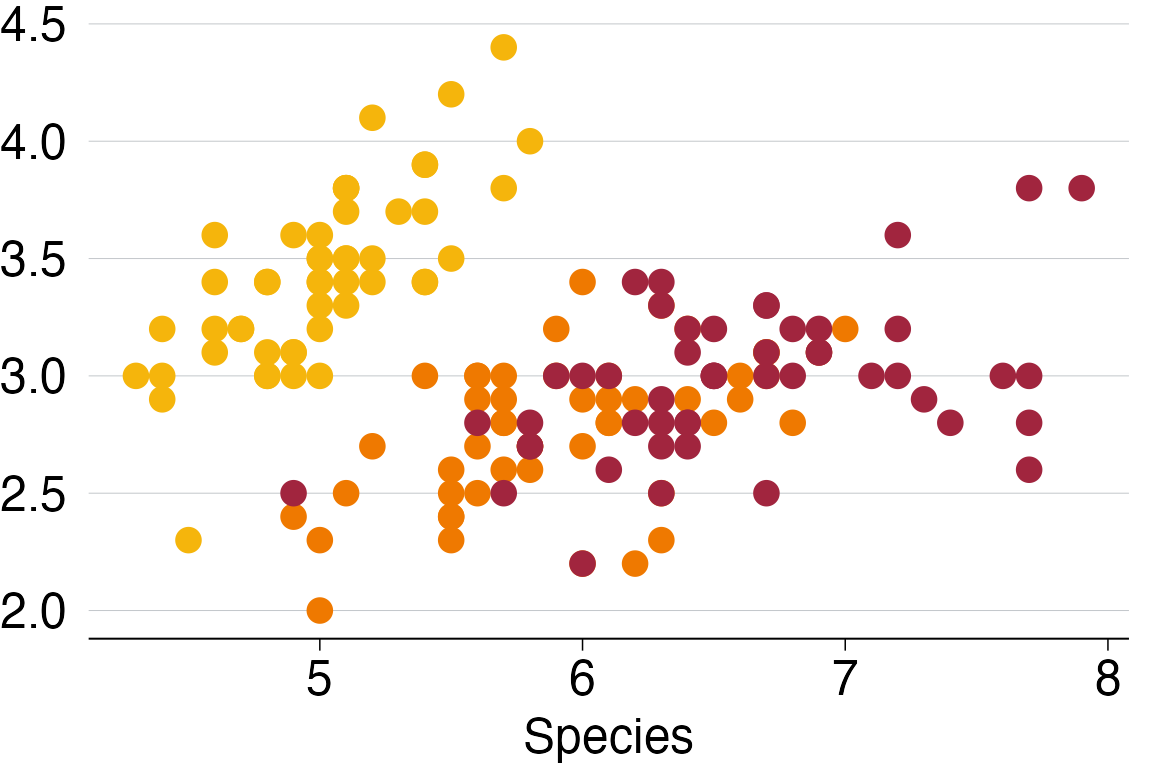

By default, theme_grattan() supresses the legend to allow for clearer on-chart labelling. We can include the legend with the legend argument, which takes "off", "top", "bottom", "left" or "right":

plot + 
  theme_grattan(legend = "top")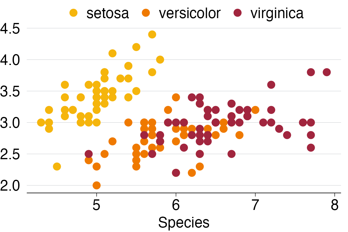

To align the y-axis with zero, change the y scale with grattan_y_continuous():

plot + 
  theme_grattan() +
  grattan_y_continuous()

Sometimes we’ll want a chart for a box in a report. We can change the background colour with the background argument:

plot + 
  theme_grattan(background = "box") +
  grattan_y_continuous()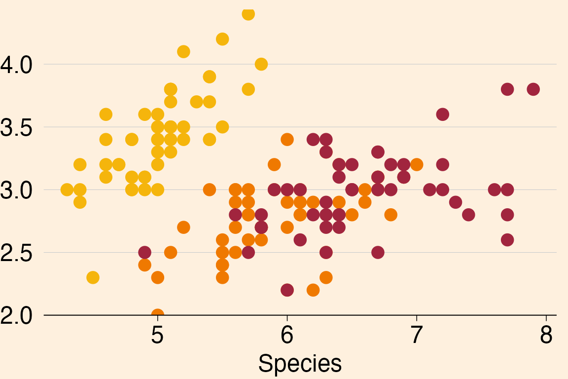

The standard Grattan rules for x and y axes flip if the chart is a horizontal bar chart. The x axis then follows the rules of the y axis, and vice-versa. If we are using a ‘flipped’ chart (imlemented with coord_flipped()), we can tell theme_grattan this is the case using the argument fillped set to TRUE.

plot + 
  coord_flip() +
  theme_grattan(flipped = TRUE) +
  grattan_y_continuous()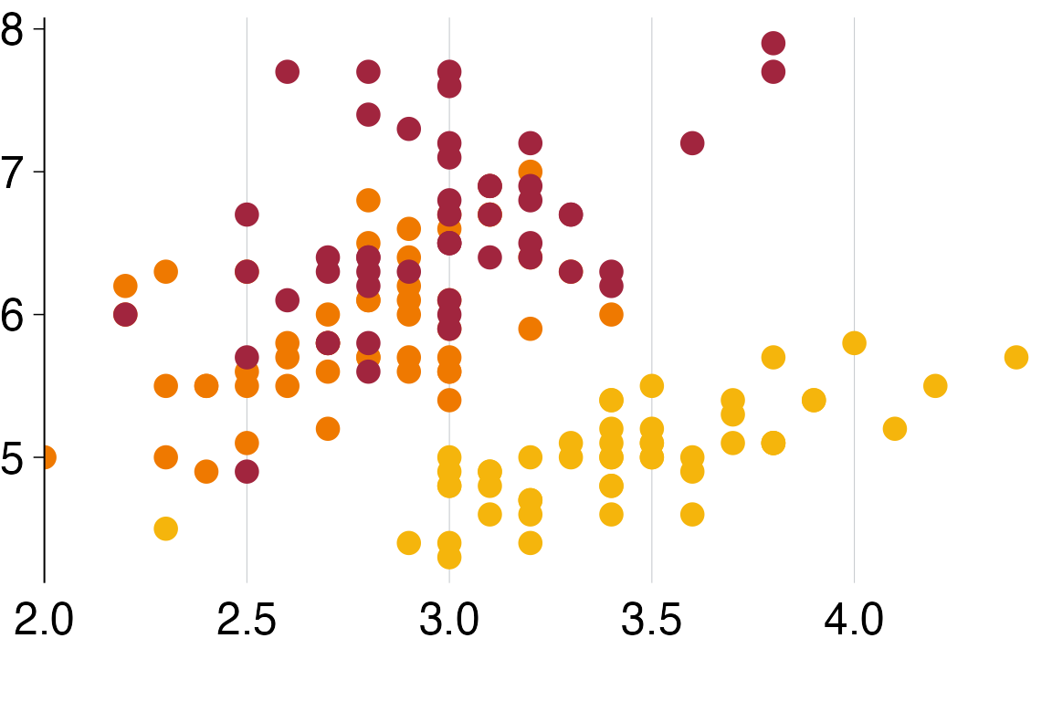

The final adjustments we can specify with theme_grattan are the font size and font family. The defaults meet Grattan formatting requirements, but if we do need to change them we can:

plot +
  theme_grattan(base_size = 8, base_family = "serif") +
  grattan_y_continuous()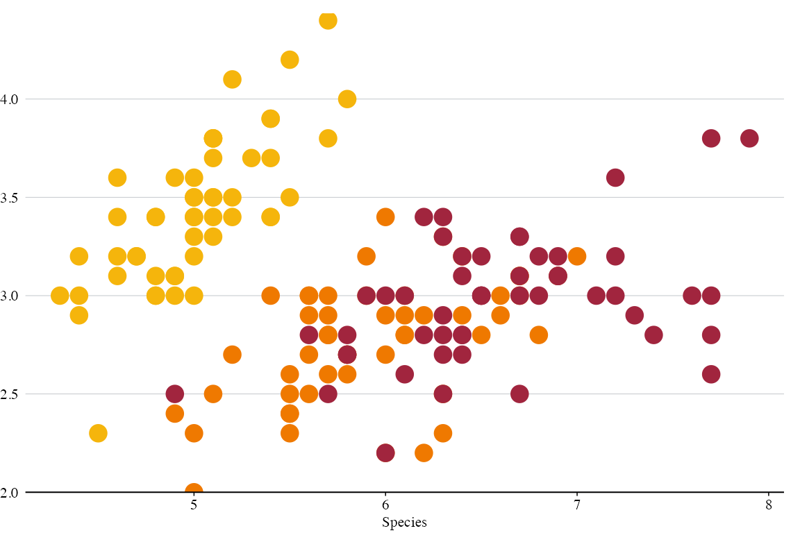

Font handling

grattantheme automatically detects and uses Grattan’s standard fonts when available: - For normal charts: uses system sans-serif fonts - For slide charts: uses DM Serif Display for titles and Avenir Next for body text

The package checks your system fonts and, if you have Dropbox synced with Grattan’s shared font folder, will automatically register fonts from there. When you load the package, you’ll see which fonts are being used.

Using Grattan colours

Grattan’s colours are loaded with grattantheme. The HEX codes for individual Grattan colours can be called using grattan_[colourname], eg grattan_lightorange. Colours names are taken from the chart-guide and are:

We can call single colours:

plot + 
  geom_hline(yintercept = 3, colour = grattan_orange) +
  geom_vline(xintercept = 6, colour = grattan_darkorange) +
  theme_grattan() +
  grattan_y_continuous()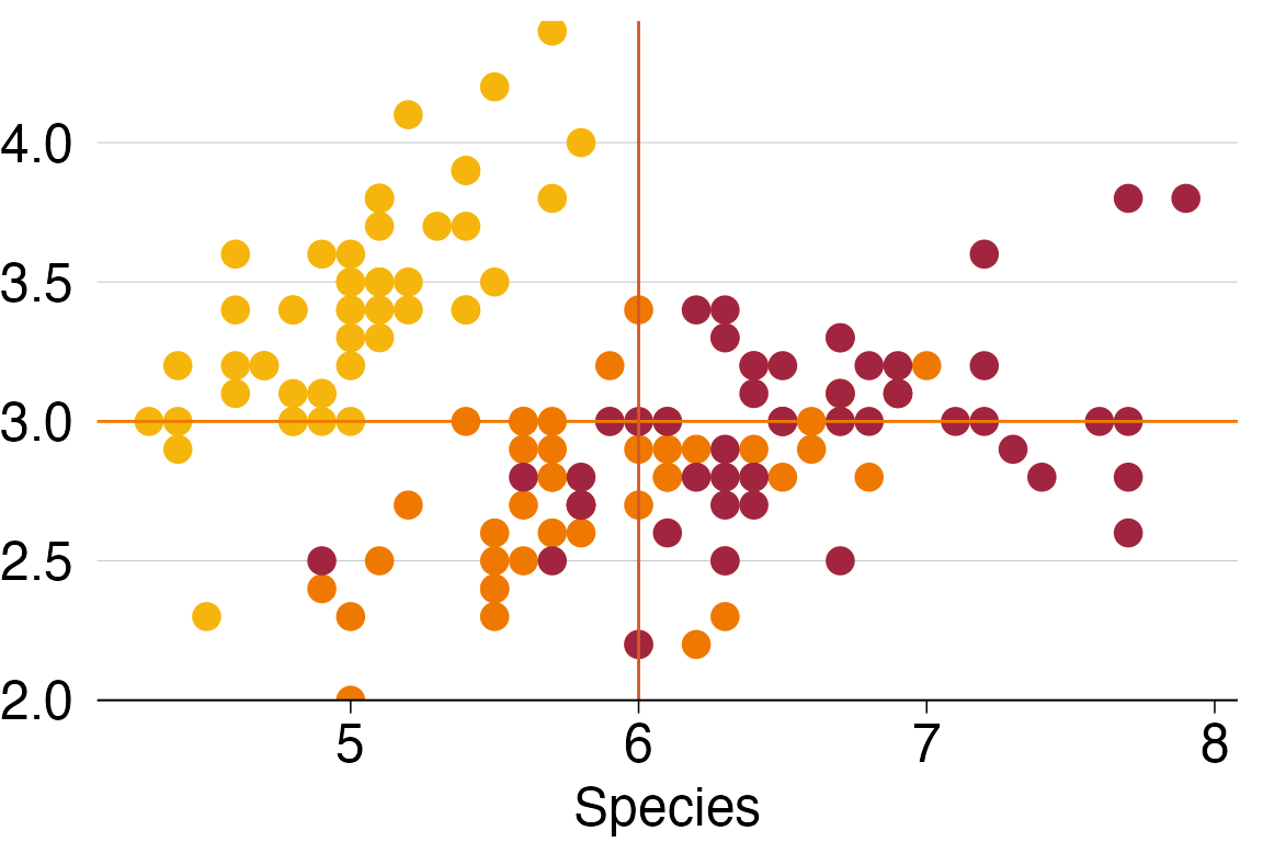

We can also use the scale_fill_grattan() or scale_colour_grattan() functions to change the colours of our fill or colour aesthetics. These can be used for discrete/catagorical data (the default) or continuous data.

Discrete colours

In our example, we have three different flowers each represented by a colour. So we need to set discrete = TRUE

plot + 
  theme_grattan() +
  grattan_y_continuous() +
  scale_colour_grattan(discrete = TRUE)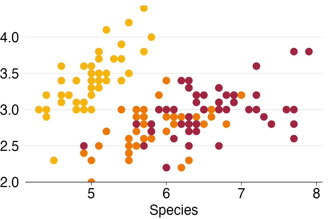

Note that if you need more than 10 colours your chart will not render some of the data. You can set a manual theme using make_grattan_pal

ggplot(mtcars, aes(x = mpg, y = hp, colour = as.character(wt))) +
  geom_point() +
  scale_colour_manual(values = make_grattan_pal()(29))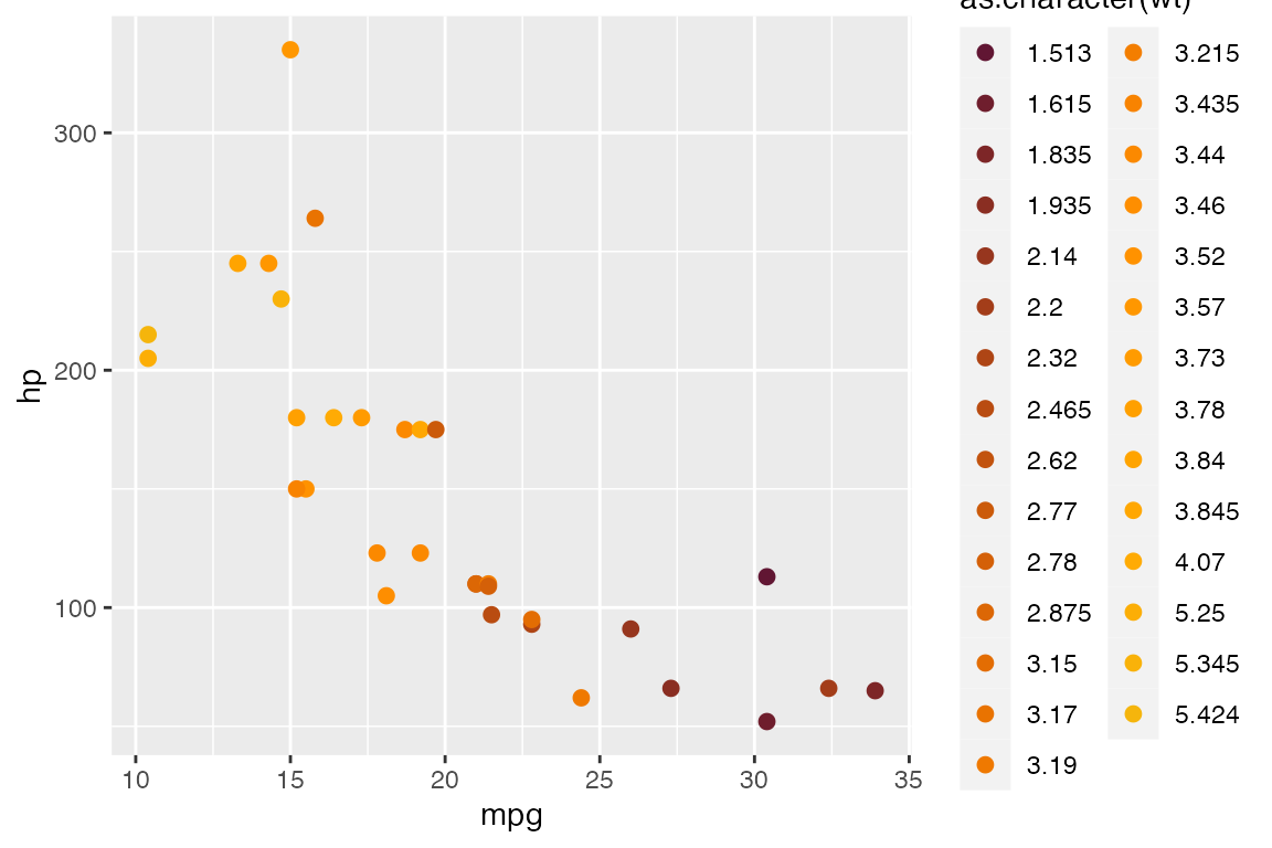

Continuous colours

scale_(colour|fill)_grattan includes an option for continuous colours: discrete = FALSE.

plot2 <- ggplot(iris,
               aes(x = Sepal.Length,
                   y = Sepal.Width,
                   colour = Sepal.Length)) +
        geom_point(size = 5) +
        scale_y_continuous_grattan() +
        labs(x = "")

plot_f <- plot2 +
  theme_grattan() +
  scale_colour_grattan(discrete = FALSE)

plot_f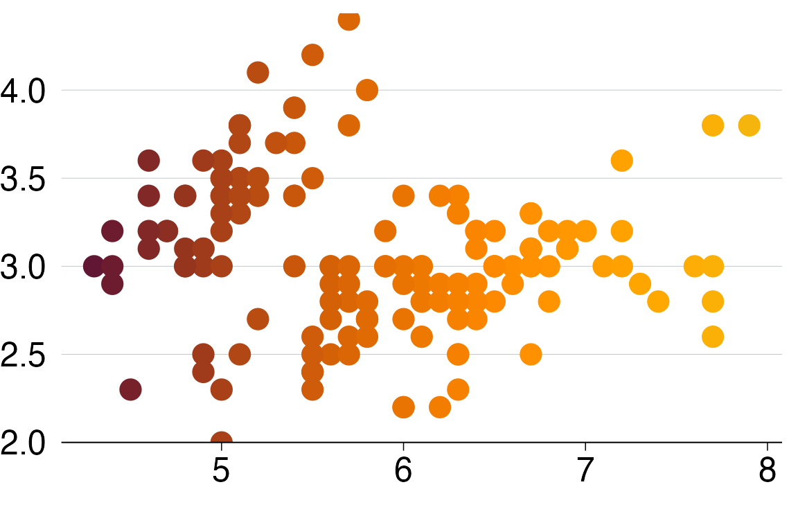

Saving plots with `grattan_save`

The grattan_save() function saves your chart in a variety of types. We specify the type with the type argument that can take the arguments:

"normal": a standard report chart size, and the default. [height = 14.5cm x width = 22.16cm]
"wholecolumn: a taller whole-column chart for reports. [22.16 x 22.16]
"fullpage": a full-page chart for reports. [22.16 x 44.32]
"fullslide" : to produce charts that look like a slide with the Grattan logo. This option allows notes and sources to accompany the saved figure.
"fullslide_narrow" : as with “fullslide”, but with a narrower chart.
"fullslide_half": as with “fullslide” but chart is half-size, with space on the right-hand side of the slide for additional annotations.

You can specify type = "all" to save in all formats.

The argument filename is required. You can specify a file extension; .pdf is standard for Grattan charts for reports and is the default if no extension is specified; .png is standard for other media.

Charts will be produced using the cairo_pdf device, unless another device is specified. Note that installation of cairo_pdf may require installation of additional software on your system, such as Xquartz on MacOS.

By default, grattan_save will save the chart in a new subdirectory that reflects the name of the chart you provide. If you wish to instead save the chart in the current working directory, you can set no_new_folder = TRUE.

grattan_save() uses the ggplot2 function ggsave() to save your chart. Like ggsave(), grattan_save() will use the last plot you displayed by default, but you can specify something else with object.

Now we can save our Grattan-formatted graph as a normally-formatted report chart:

# Create and store the plot:
plot_final <- plot_f +
              labs(title = "Iris plants are rad!",
                 subtitle = "Width of sepal",
                 x = "Length of sepal", 
                 y = "",
                 caption = "Notes: A classic dataset. Source: Fisher (1936)")

# Save the plot
grattan_save(filename = "iris.pdf",
             object = plot_final,
             type = "normal")
#> Warning in grSoftVersion(): unable to load shared object '/Library/Frameworks/R.framework/Resources/modules//R_X11.so':
#>   dlopen(/Library/Frameworks/R.framework/Resources/modules//R_X11.so, 0x0006): Library not loaded: /opt/X11/lib/libSM.6.dylib
#>   Referenced from: <7ECC4104-EC6A-38FD-9BEA-BFE0B870925C> /Library/Frameworks/R.framework/Versions/4.5-arm64/Resources/modules/R_X11.so
#>   Reason: tried: '/opt/X11/lib/libSM.6.dylib' (no such file), '/System/Volumes/Preboot/Cryptexes/OS/opt/X11/lib/libSM.6.dylib' (no such file), '/opt/X11/lib/libSM.6.dylib' (no such file), '/Library/Frameworks/R.framework/Resources/lib/libSM.6.dylib' (no such file), '/Users/runner/hostedtoolcache/Java_Temurin-Hotspot_jdk/21.0.9-10.0/arm64/Contents/Home//lib/server/libSM.6.dylib' (no such file), '/Library/Frameworks/R.framework/Resources/lib/libSM.6.dylib' (no such file), '/Users/runner/hostedtoolcache/Java_Temurin-Hotspot_jdk/21.0.9-10.0/arm64/Contents/Home//lib/server/libSM.6.dylib' (no such file)
#> Warning in cairoVersion(): unable to load shared object '/Library/Frameworks/R.framework/Resources/library/grDevices/libs//cairo.so':
#>   dlopen(/Library/Frameworks/R.framework/Resources/library/grDevices/libs//cairo.so, 0x0006): Library not loaded: /opt/X11/lib/libXrender.1.dylib
#>   Referenced from: <263B701F-2238-3478-A7D2-B7513231EF98> /Library/Frameworks/R.framework/Versions/4.5-arm64/Resources/library/grDevices/libs/cairo.so
#>   Reason: tried: '/opt/X11/lib/libXrender.1.dylib' (no such file), '/System/Volumes/Preboot/Cryptexes/OS/opt/X11/lib/libXrender.1.dylib' (no such file), '/opt/X11/lib/libXrender.1.dylib' (no such file), '/Library/Frameworks/R.framework/Resources/lib/libXrender.1.dylib' (no such file), '/Users/runner/hostedtoolcache/Java_Temurin-Hotspot_jdk/21.0.9-10.0/arm64/Contents/Home//lib/server/libXrender.1.dylib' (no such file), '/Library/Frameworks/R.framework/Resources/lib/libXrender.1.dylib' (no such file), '/Users/runner/hostedtoolcache/Java_Temurin-Hotspot_jdk/21.0.9-10.0/arm64/Contents/Home//li [... truncated]
#> Warning in device(filename = "iris/iris_normal.pdf", width = 8.7244094488189, :
#> failed to load cairo DLL

Which produces a chart that can fit into a report. Note that the title, subtitle and notes/sources have been removed.

Saving Powerpoint files

It’s convenient to also save your files in Powerpoint format. This allows PDs to easily use your graphs in their presentations. Saving in this format also means you can include speaker notes – such as information about the script used to create the file – which can help us to keep track of things.

You can save a Powerpoint file, with appropriate speaker notes included, like this:

grattan_save("iris_fullslide.pdf",
             plot_final,
             type = "fullslide",
             save_pptx = TRUE)

Or, you can use the grattan_save_pptx function, like this:

grattan_save_pptx(plot_final,
                  "iris_fullslide.pptx",
                  type = "fullslide")

Note that the grattan_save_pptx function does not create a new subdirectory for your file, while grattan_save will by default, unless no_new_folder is set.

If your chart includes markdown-formatted text either in chart labels or in the chart subtitle, officer will often fail to correctly format the Powerpoint slide output. As a workaround, you can use the option rich_subtitle = T, which converts both your chart and subtitle to a .png file, which is inserted into the Powerpoint slide. This means the content (including fonts) cannot then be edited in Powerpoint after the fact , but will correctly reflect any markdown formatting.

Saving chart data

When we release reports or working papers, we typically upload an Excel file including ‘chart data’ for most of our charts. The process for making and properly formatting these files can be a bit laborious. grattantheme helps streamline that process, using the save_chartdata() function.

You can use it like this:

grattan_save("plot_final.png",
             type = "fullslide",
             save_data = TRUE)

Or you can use the save_chartdata function directly, like this:

save_chartdata("plot_final.xlsx", object = plot_final)

Saving to an Overleaf atlas

Grattan reports are drafted in Overleaf, with charts saved to an ‘atlas’ folder. Once this folder has been set up to sync locally via Dropbox, you can save charts directly from R to your Overleaf project using grattan_save_overleaf().

The first time you use grattan_save_overleaf() in an R session, you’ll be prompted to select which Overleaf project to use from those synced in your Dropbox. Your choice is stored for the current R session only.

For reproducibility, we recommend setting your Overleaf project at the start of your script:

library(grattantheme)

# Set the Overleaf project
set_overleaf_project("Orange-Book-2025")  # Searches for matching project name

# Create and save your chart
plot_final <- ggplot(mtcars, aes(x = wt, y = mpg)) + 
  geom_point() +
  theme_grattan()

grattan_save_overleaf("my_chart.pdf", plot_final)

The function saves only the PDF version of your chart to the atlas folder. No subfolders, PowerPoint slides, or chart data files are created. You can still specify chart types:

# Save as a taller chart
grattan_save_overleaf("tall_chart.pdf", plot_final, type = "wholecolumn")

To change which project you’re saving to during your session:

set_overleaf_project("transport-report")
grattan_save_overleaf("another_chart.pdf", plot_final)

Formatting theme elements with theme_grattan()