4 Grattan’s coding style and the tidyverse
The benefits of a common coding style are well explained by Hadley Wickham:
Good style is important because while your code only has one author, it’ll usually have multiple readers. This is especially true when you’re writing code with others. In that case, it’s a good idea to agree on a common style up-front.
Below we describe the key elements of Grattan coding style, without being too tedious about it all. There are many elements of coding style we don’t cover in this guide; if you’re unsure about anything, consult the tidyverse guide.
You should also see the Using R at Grattan page for guidelines about setting up your project.
A core principle for coding at Grattan is that your code should be readable by humans. For this reason, we prefer to use the tidyverse set of packages for data reading, manipulation and visualisation.
4.1 The tidyverse

The tidyverse is central to our work at Grattan. The tidyverse is a collection of related R packages for importing, wrangling, exploring and visualising data in R. The packages are designed to work well together.
4.1.1 Why do we use the tidyverse?
The tidyverse makes life easier!
The core tidyverse packages, like ggplot2, dplyr, and tidyr, are extremely popular. The tidyverse is probably the most popular ‘dialect’ of R. This means that any problem you encounter with the tidyverse will have been encountered many times before by other R users, so a solution will only be a Google search away.
The tidyverse packages are all designed to work well together, with a consistent underlying philosophy and design. This means that coding habits you learn with one tidyverse package, like dplyr, are also applicable to other packages, like tidyr.
They’re designed to work with data frames17, a rectangular data object that will be familiar to spreadsheet users that is very intuitive and convenient for the sort of work we do at Grattan. In particular, the tidyverse is built around the concept of tidy data, which has a specific meaning in this context that we’ll come to later. The fact that tidyverse packages are all built around one type of data object makes them easier to work with.
The creator of the tidyverse, Hadley Wickham, places great value on code that is expressive and comprehensible to humans. This means that code written in the tidyverse idiom is often able to be understood even if you haven’t encountered the functions before. For example, look at this chunk of code:
Without knowing what my_data looks like, and even if you haven’t encountered these functions before, this should be reasonably intuitive. We’re taking some data, and then18 only keeping observations that relate to people aged 30 and older, then calculating a new variable, relative_income. The name of a tidyverse function - like filter, group_by, summarise, and so on - generally gives you a pretty good idea what the function is going to do with your data, which isn’t always the case with other approaches.
Here’s one way to do the same thing in base R:
The base R code gets the job done, but it’s clunkier, less expressive, and harder to read. A core principle of coding at Grattan is that you should strive to make your work human readable.
Code written with tidyverse functions is often faster than its base R equivalents. But most of our work at Grattan is with small-to-medium sized datasets (with fewer than a million rows or so), so speed isn’t usually a major concern anyway.19
The most valuable resource we deal with at Grattan is our time. Computers are cheap, people are not. If your code executes quickly, but it takes your colleague many hours to decipher it, the cost of the extra QC time more than outweighs the saving through faster computation. The tidyverse packages strike a balance between expressive, comprehensible code and computational efficiency that suits the nature of our work at Grattan. This balance is the right one for most of our work, most of the time.
Most R scripts at Grattan should start with library(tidyverse). Most of your work will be in data frames, and most of the time the tidyverse contains the core tools you’ll need to do that work.
4.2 Load packages first
Our analysis scripts will almost always involve loading some packages. These should be laoded at the top of a script, in one block like this:
If you’re loading a package from Github, it’s a good idea to leave a comment to say where it came from, like this:
library(tidyverse)
library(grattantheme) # remotes::install_github("grattan/grattantheme")
library(strayr) # remotes::install_github("runapp-aus/strayr")Don’t scatter library() calls throughout your script - put them all at the top.
The only thing that should come before loading your packages is the script preamble.
4.3 Script preamble
Describe what your script does in the first few lines using comments or within an RMarkdown document.
Good
# This script reads ABS data downloaded from TableBuilder and combines into a single data object containing post-secondary education levels by age and gender by SA3. Your preamble might also pose a research question that the script will answer.
Good
# Do women have higher levels of educational attainment than men, within the same geographical areas and age groups?Your preamble shouldn’t be a terse, inscrutable comment.
Bad
# make ABS ed data graphIf it’s hard to concisely describe what your script does in a few lines of plain English, that might be a sign that your script does too many things. Consider breaking your analysis into a series of scripts. See Organising R Projects at Grattan for more.
Your preamble should anticipate and answer any questions other people might have when reviewing your script. For example:
Good
# This script calculates average income by age group and sex using the ABS Household Expenditure Survey and joins this to health information by age groups and sex from the National Health Survey. Note that we can't use the income variable in the NHS for this purpose, as it only contains information about respondents' income decile, not the income itself.The preamble should pertain the the code contained in the specific script. If you have comments or information about your analysis as a whole, put it in your README file.
4.4 Use comments
Comments are necessary where the code alone doesn’t tell the full story. Comments should tell the reader why you’re doing something, rather than just what you’re doing.
For example, comments are important when groups are coded with numbers rather than character strings, because this might not be obvious to someone reading your script:
Necessary to comment
data %>%
  filter(gender == 1,   # Keep only male observations
         age == "05")   # Keep only 35-39 year-olds.
Without the comment, readers of your code might not be aware that 1 in this dataset corresponds to male, or that age == "05" refers to 35-39 year olds. Without the comment, the code is not self-explanatory.
If your code is self-explanatory, you can include or omit comments as you see fit.
Not necessary (but okay if included)
# We want to only look at women aged 35-39
data %>%
  filter(gender == "Female",
         age >= 35 & age <= 39)
You should also include comments where your code is more complex and may not be easily understood by the reader. If you’re using a function from a package that isn’t commonly used at Grattan, include a comment to explain what it does.
Err on the side of commenting more, rather than less, throughout your code. Something may seem obvious to you when you’re writing your code, but it might not be obvious to the person reading your code, even if that person is you in the future. Better to over-comment than under-comment.
Comments can go above code chunks, or next to code - there are examples of both above.
 ## Breaking your script into chunks
It’s useful to break a lengthy script into chunks with ----- (three or more hyphens).
Good
# Read file A -----

a <- read_csv("data/a.csv")

# Read file B -----

b <- read_csv("data/b.csv")

# Combine files A and B ----

c <- bind_rows(a, b)
(In practice, you’ll have more than one line of code in each block.)
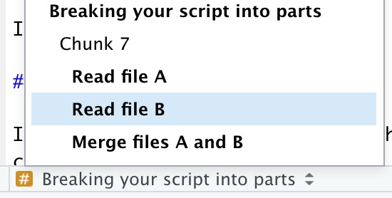
This helps you, and others, navigate your code better, using the navigation tool built in to RStudio. In the script editor pane of RStudio, at the bottom left, there’s a little navigation tool that helps you easily jump between named sections of your script.
Breaking your script into chunks with ----- also makes your code easier to read.
4.5 Assigning values to objects
In R, you work with objects. An object might be a data frame, or a vector of numbers or letters, or a list. Functions can be objects, too.
Use the <- operator to assign values to objects. Here are some good examples:
schools <- read_csv("data/schools_data.csv")

three_letters <- c("a", "b", "c")

lf <- labour_force %>%
  filter(status != "NILF")
Avoid ->, = and assign(). Here are some bad examples::
schools = read_csv("data/schools_data.csv")

assign("three_letters", c("a", "b", "c"))

labour_force %>%
  filter(status != "NILF") -> lf
All these bad operators will work, but they are best avoided. The = operator is avoided for reasons of visual consistency, style, and to avoid confusion. assign() is avoided because it can lead to unexpected behaviour, and is usually not the best way to do what you want to do. The -> operator is avoided because it’s easy to miss when skimming over code.
The <<- operator should also be avoided.
4.6 Naming objects and variables
It’s important to be consistent when naming things. This saves you time when writing code. If you use a consistent naming convention, you don’t need to stop to remember if your object is called ed_by_age or edByAge or ed.by.age. Having a consistent naming convention across Grattan also makes it easy to read and QC each other’s code.
Grattan uses words separated by underscores _ (aka ‘snake_case’) to name objects and variables. This is common practice across the Tidyverse.
Object names should be descriptive and not-too-long. This is a trade-off, and one that’s sometimes hard to get right. However, using snake_case provides consistency:
Good object names
sa3_population
gdp_growth_vic
uni_attainment
Bad object names
sa3Pop
GDPgrowthVIC
uni.attainment
Variable names face a similar trade-off. Again, try to be descriptive and short using snake_case:
Good variable names
gender
gdp_growth
highest_edu
Bad variable names
s801LHSAA
gdp.growth
highEdu
chaosVar_name.silly
var2
When you load data from outside Grattan, such as ABS microdata, variables will often have bad names. It is worth taking the time at the top of your script to rename your variables, giving them consistent, descriptive, short, snake_case names. An easy way to do this is using clean_names() function from the janitor package:
df_with_bad_names <- data.frame(firstColumn = c(1:3),
                                Second.column = c(4:6))

df_with_good_names <- janitor::clean_names(df_with_bad_names)

df_with_good_names
## first_column second_column
## 1 1 4
## 2 2 5
## 3 3 6The most important thing is that your code is internally consistent - you should stick to one naming convention for all your objects and variables. Using snake_case, which we strongly recommend, reduces friction for other people reading and editing your code. Using short names saves effort when coding. Using descriptive names makes your code easier to read and understand.
4.7 Spacing
Giving your code room to breathe greatly helps readability for future-you and others who will have to read your code. Code without ample whitespace is hard to read, justasitishardertoreadEnglishsentenceswithoutspaces.
4.7.1 Assign and equals
Put a space each side of an assign operator <-, equals =, and other ‘infix operators’ (==, +, -, and so on).
Good
uni_attainment <- filter(data, age == 25, gender == "Female")Bad
uni_attainment<-filter(data,age==25,gender=="Female")Exceptions are operators that directly connect to an object, package or function, which should not have spaces on either side: ::, $, @, [, [[, etc.
Good
uni_attainment$gender
uni_attainment$age[1:10]
readabs::read_abs()
Bad
uni_attainment $ gender
uni_attainment$ age [ 1 : 10]
readabs :: read_abs()
4.7.2 Commas
Always put a space after a comma and not before, just like in regular English.
Good
select(data, age, gender, sa2, sa3)Bad
4.7.3 Parentheses
Do not use spaces around parentheses in most cases:
Good
mean(x, na.rm = TRUE)Bad
For spacing rules around if, for, while, and function, see the Tidyverse guide.
4.8 Short lines, line indentation and the pipe %>%
Keeping your lines of code short and indenting them in a consistent way can help make reading code much easier. If you are supplying multiple arguments to a function, it’s generally a good idea to put each argument on a new line - hit enter/return after the comma, like in the rename and filter examples below. Indentation makes it clear where a code block starts and finishes.
Using pipes (%>%) instead of nesting functions also makes things clearer.20 The pipe should always have a space before it, and should generally be followed by a new line, as in this example:
Good: short lines and indentation
young_qual_income <- data %>%
  rename(gender = s801LHSAA,
         uni_attainment = high.ed) %>%
  filter(income > 0,
         age >= 25 & age <= 34) %>%
  group_by(gender,
           uni_attainment) %>%
  summarise(mean_income = mean(income,
                               na.rm = TRUE))
Without indentation, the code is harder to read. It’s not clear where the chunk starts and finishes, and which bits of code are arguments to which functions.
Bad: short lines, no indentation
young_qual_income <- data %>%
rename(gender = s801LHSAA,
uni_attainment = high.ed) %>%
filter(income > 0,
age >= 25 & age <= 34) %>%
group_by(gender, uni_attainment) %>%
summarise(mean_income = mean(income, na.rm = TRUE))
Long lines are also bad and hard to read. Bad: long lines
young_qual_income <- data %>% rename(gender = s801LHSAA, uni_attainment = high.ed) %>% filter(income > 0, age >= 25 & age <= 34) %>% group_by(gender, uni_attainment) %>% summarise(mean_income = mean(income, na.rm = TRUE))When you want to take the output of a function and pass it as the input to another function, use the pipe (%>%). Don’t write ugly, inscrutable code like this, where multiple functions are wrapped around other functions.
War-crime bad: long lines without pipes
young_qual_income<-summarise(group_by(filter(rename(data,gender=s801LHSAA,uni_attainment=high.ed),income>0,age>=25&age<=34),uni_attainment),mean_income=mean(income,na.rm=TRUE))Writing clear code chunks, where functions are strung together with a pipe (%>%), makes your code much more expressive and able to be read and understood. This is another reason to favour R over something like Excel, which pushes people to piece together functions into Frankenstein’s monsters like this:
=IF($G16 = "All day", INDEX(metrics!$D$8:$H$66, MATCH(INDEX(correspondence!$B$2:$B$23, MATCH('convert to tibble'!M$4, correspondence!$A$2:$A$23, 0)), metrics!$B$8:$B$66, 0), MATCH('convert to tibble'!$E16, metrics!$D$4:$H$4, 0)), "NA")I just threw up in my mouth a little bit.
The pipe function %>% can make code more easy to write and read. The pipe can create the temptation to string together lots and lots of functions into one block of code. This can make things harder to read and understand.
Resist the urge to use the pipe to make code blocks too long. A block of code should generally do one thing, or a small number of things.
4.9 Omit needless code
Don’t retain code that ultimately didn’t lead anywhere. If you produced a graph that ended up not being used, don’t keep the code in your script - if you want to save it, move it to a subfolder named ‘archive’ or similar. Your code should include the steps needed to go from your raw data to your output - and not extraneous steps. If you ask someone to QC your work, they shouldn’t have to wade through 1000 lines of code just to find the 200 lines that are actually required to produce your output.
When you’re doing data analysis, you’ll often give R interactive commands to help you understand what your data looks like. For example, you might view a dataframe with View(mydf) or str(mydf). This is fine, and often necessary, when you’re doing your analysis. Don’t keep these commands in your script. These type of commands should usually be entered straight into the R console, not in a script. If they’re in your script, delete them.