2 Getting started

This chapter gets you up and running with R Studio and writing R code like a real hacker.

Goals: By the end of this chapter you will have R and R Studio installed, and be able to write, execute and understand some simple R code.

2.1 Installing R and RStudio

Although you’ll usually work with R by opening RStudio, you need to install both R and RStudio separately.

Install R by going to CRAN, the Comprehensive R Archive Network. CRAN is a community-run website that houses R itself as well as a broad range of R packages.

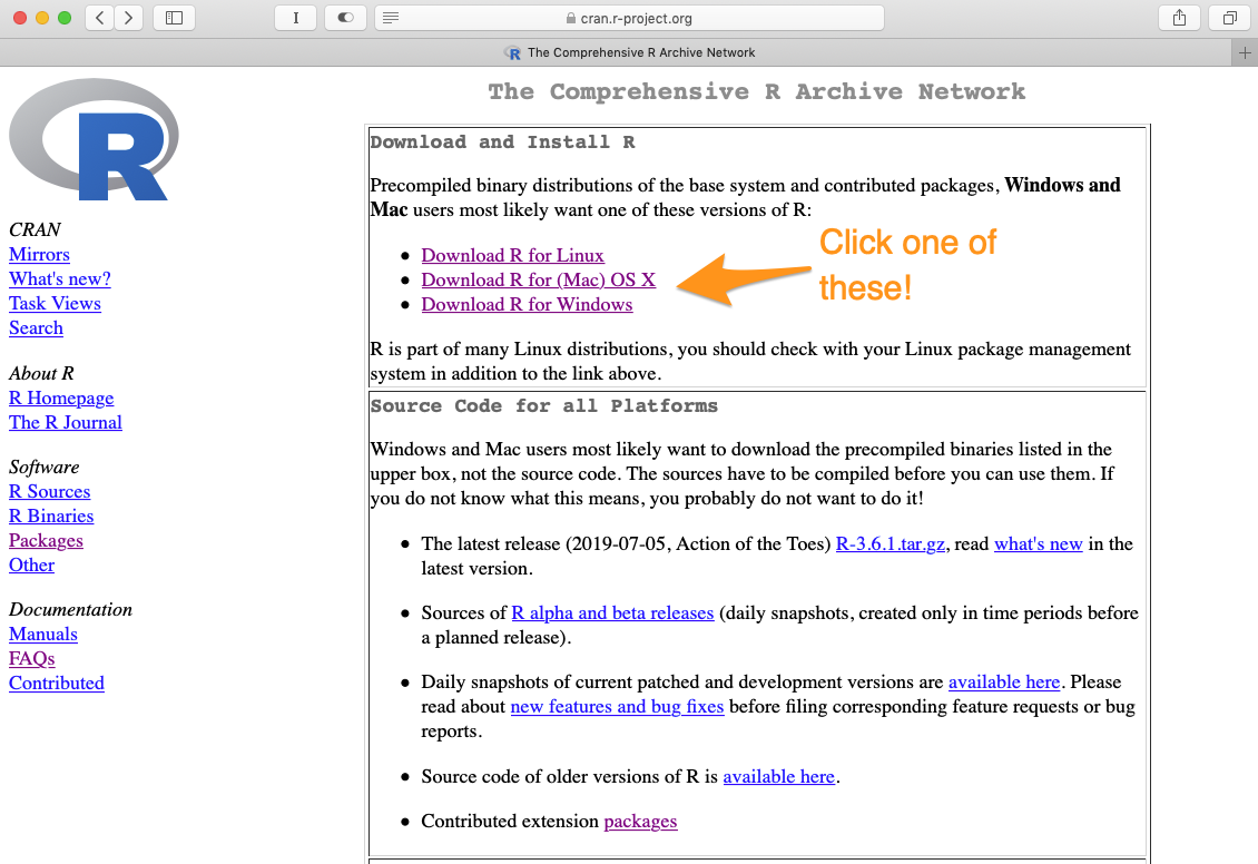
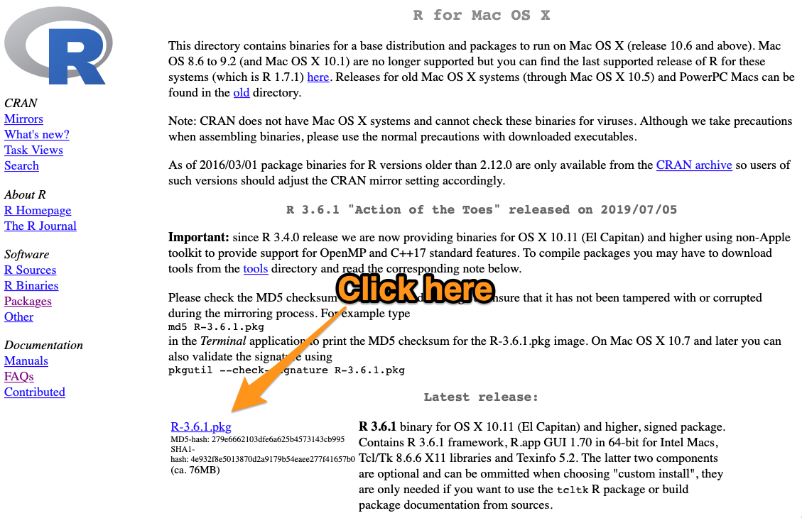
You want to download the latest base R release, as a ‘binary’. Don’t worry, you don’t need to know what a binary is.

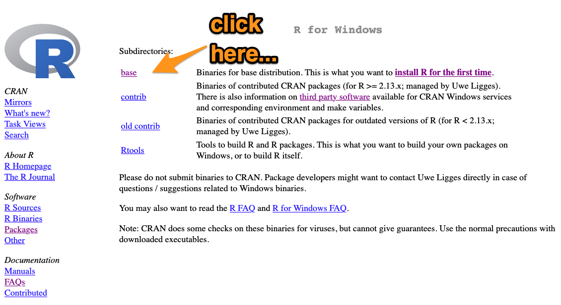
For macOS, the page will look like this:

For Windows, you’ll need to click on the ‘base’ version, and then click again to start the download.

Once you’ve installed R, you’ll need to install RStudio. Go to the RStudio website and install the latest version of RStudio Desktop (open source license).

Once they’re both installed, get started by opening RStudio.

2.2 Setting up RStudio

Change the defaults of Rstudio to make it a bit easier to use.

Open your R studio preferences by:

# install the package 
install.packages("usethis")

# open your R preferences
usethis::edit_rstudio_prefs()

And then copy the following, updating the relevant bits.

{
    "default_project_location": "C:/r_projects",
    "soft_wrap_r_files": true,
    "scroll_past_end_of_document": true,
    "highlight_r_function_calls": true,
    "save_files_before_build": true,
    "editor_theme": "Tomorrow",
    "default_encoding": "UTF-8",
    "document_author": "tyler reysenbach",
    "wrap_tab_navigation": false,
    "save_workspace": "never",
    "rainbow_parentheses": true,
    "reuse_sessions_for_project_links": true,
    "syntax_color_console": true,
    "spelling_dictionary_language": "en_AU",
    "windows_terminal_shell": "win-git-bash",
    "jobs_tab_visibility": "shown",
    "cran_mirror": {
        "name": "Australia (Canberra) [https]",
        "host": "CSIRO",
        "url": "http://cran.csiro.au/",
        "secondary": "",
        "country": "au"
    },
    "graphics_backend": "cairo",
    "graphics_antialiasing": "subpixel",
    "console_double_click_select": true,
    "load_workspace": false,
    "knit_working_dir": "project",
    "doc_outline_show": "sections_and_chunks",
    "rmd_viewer_type": "pane",
    "rmd_chunk_output_inline": false,
    "use_internet2": false,
    "show_publish_diagnostics": true,
    "use_secure_download": false,
    "initial_working_directory": "~",
    "source_with_echo": true
}

2.3 Scripts and ‘coding’

R is a script-based program. You write a list of instructions and R will follow it. This is wonderfully handy:

everything you have told it to do, it will do;
you have a record of everything you have told it to do.

But ‘coding’ can intimidating! However, it’s just a list of instructions. If you have ever used Excel you have used functions to create output. You have written code. You’re already a coder!

We can greatly enhance the things we can do by using R. The rest of this chapter is a short guide to walk you through your first lines of R code. If you get stuck or something doesn’t work or you have an urge to throw your computer out the window, please reach out to Will or James, or post on the #r_at_grattan Slack channel, and someone will help you out.

2.4 A practical introduction to writing R code

2.4.1 Starting a new script and defining an object

From within RStudio, open a new script by: File -> New File -> R Script.

In that script, let’s do three things:

Write a comment starting with # something R will ignore – it’s just there for you.
Define an object: assign the number 119 to the object named goodnumber.⁴ We assign something in R by using <-, which you can read as ‘assign the thing on the right to the objected on the left’.⁵
Calculate a thing.

Your script will look like this:

# Hello I am starting my R script

goodnumber <- 119

2 * goodnumber

## [1] 238

The code that you write in your script will sit there idly until you send it to be processed in the console. Run the code by:

sending the current line (where your cursor is) to the console with keyboard shortcut CMD + return (Mac) or CTRL + shift (Windows); or
selecting a few lines of code and sending it to the console with the same keyboard shortcut; or
running the whole script – from the first line to the last – clicking ‘Run’:

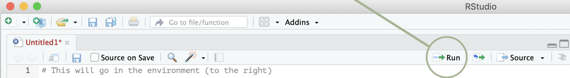
Having run your three lines of code, your RStuido should now look something like this:

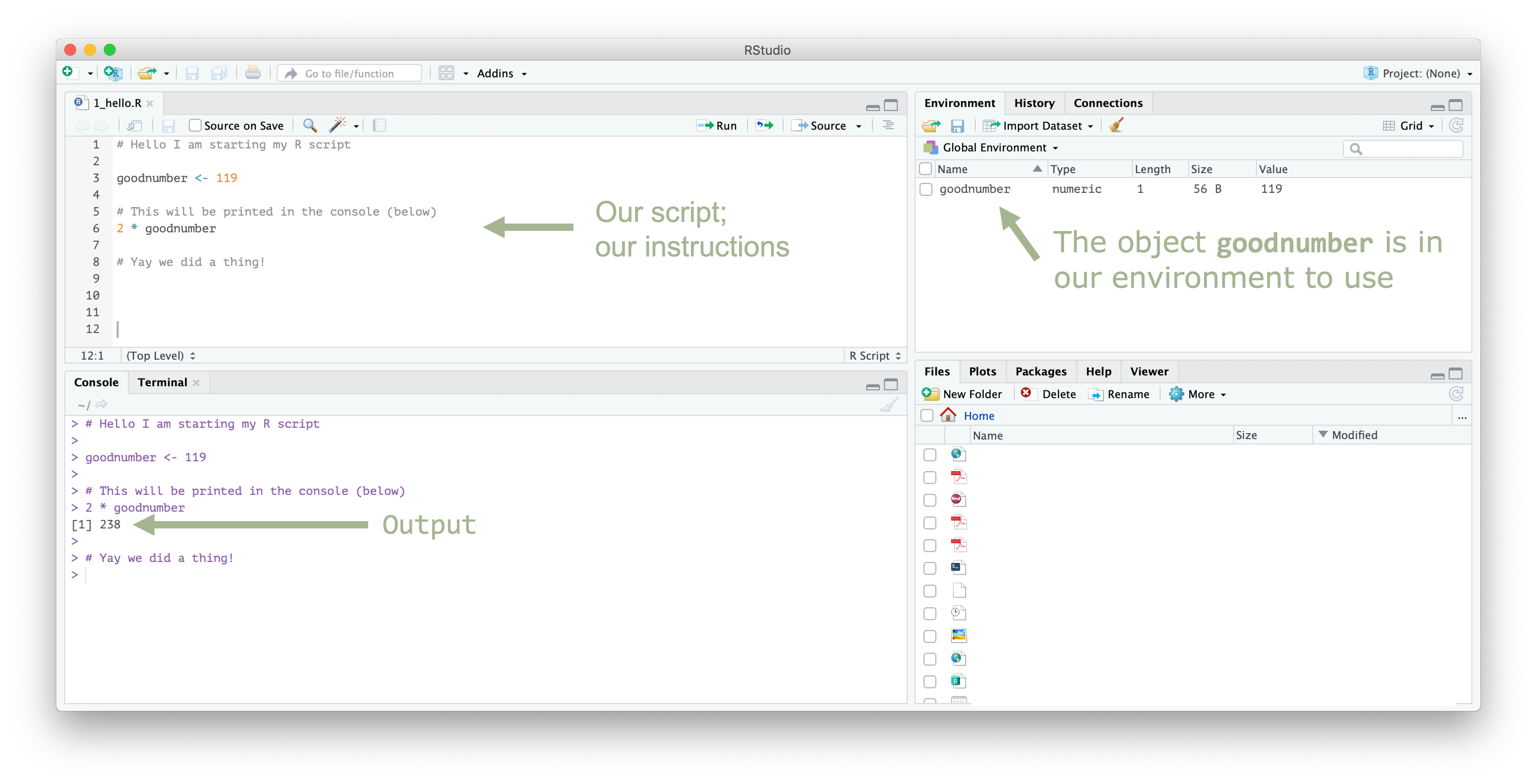
The object are stored in your environment (top-right panel of your RStudio window). You can think about your environment as the things that R knows about at this point in time.

Exercise 1:

In your R script:

Define an object to be equal to 90
Multiply the object by 100
Divide the object by 10
Why does the final step produce 9 (90 / 10) rather than 900 ((90 * 100) / 10)?
How might you incorporate the second line into your code so that the result is 900 as described above?

Answer:

cool_object <- 90

cool_object * 100

## [1] 9000

cool_object / 10

## [1] 9

The final line cool_object / 10 results in 9 because we have defined cool_object to be 90 in the first line of code, but not assigned the second line of code cool_object * 90 to an object.

To incorporate the second line we would need to define cool_object or use a different object to then be used in the third line:

cool_object <- 90

new_object <- cool_object * 100
new_object

## [1] 9000

new_object / 10

## [1] 900

2.4.2 Functions

A function takes inputs (arguments, or parameters), performs an operation (or many), and produces outputs. For example, we can use the c function to combine numbers into a series of numbers (called a vector):

c(3, 4, 5)

## [1] 3 4 5

‘combine the elements 3, 4 and 5 into a single vector’

You could combine this with the mean function that calculates the average by ‘nesting’ one function inside another:⁶

mean(c(3, 4, 5))

## [1] 4

Above, R will first process the c command that combines the numbers into a single vector, c(3, 4, 5), and then process the mean command which takes the average of the numbers in that vector. In other words, it runs inside out.

But we aren’t very good at reading things inside out, and so writing things this way can quickly become difficult. By assigning the vector to an object with <-, you could instead write your script so it first combines the numbers into a vector, and then takes the mean of that vector:⁷

goodnumbers <- c(3, 4, 5)
mean(goodnumbers)

## [1] 4

Hot tip: if you want to know more information about a function you can access its documentation by asking R. Type ? followed by the function name – e.g. ?mean – into the console and a handy little help window will pop up in the bottom right of your RStudio window.

This is a useful exercise when you’re trying to remember what the function needs as inputs (parameters, or arguments), what the function actually does, or what the function outputs.

Try these in your own console:

?mean
?median
?max

You could then apply different functions to that same set of numbers:

median(goodnumbers)

## [1] 4

sd(goodnumbers)

## [1] 1

max(goodnumbers)

## [1] 5

min(goodnumbers)

## [1] 3

2.4.3 Data types

Data ‘types’ define how your data is stored and what you can (or cannot) do with it.⁸ A piece of data might be a:

numeric: a number, like 6
a character: characters within quotation marks, like “hello”.
a logical: binary TRUE or FALSE, and nothing in between.

These types are important. As we have seen above, you can do maths on numbers:

num1 <- 10
num2 <- 5

num1 + num2

## [1] 15

num1 / num2

## [1] 2

And you can perform string operations on characters:

char1 <- "Hello"

substring(char1, 4, 6)

## [1] "lo"

But you can’t perform maths on characters, because that doesn’t really make sense:

"Hello" * 2

## Error in "Hello" * 2: non-numeric argument to binary operator

Even when you kind of think it should:

"100" * 2

## Error in "100" * 2: non-numeric argument to binary operator

Above, R is trying to multiply the character "100" by the number 2. Which – because of the types of these data – makes as much sense as "Hello" \(\times\) 2.

We can use in-built functions to change the class of an object. To solve our issue above, we could convert "100" into a numeric before we do cool maths on it:

as.numeric("100") * 2

## [1] 200

Cool!

2.4.4 Errors, warnings and messages

When you run your code, there are three types of things that will pop up in response in addition to any output you might expect:

Message (hello)
Warning (warning!)
Error message (oh no!)

Messages are friendly and are designed to just keep you abreast with what’s going on. Messages are not prefixed with anything, they’ll just pop up as you’re running a function. How ‘verbose’ a function it is – how much it talks to you via messages – will depend on the authors. An example of a message is below:

message("Just typing R code, all good")

## Just typing R code, all good

Warnings indicate that there is something you should be aware of. The function still runs and your output will still be produced, but something might be off. A warning message will be prefixed with Warning message:. For example:

warning("Ooooh something could be wrong here and I just thought you should know about it.")

## Warning: Ooooh something could be wrong here and I just thought you should know
## about it.

A classic example of a warning message is when the as.numeric() function we saw in the previous section encounters a character it just can’t find a suitable corresponding number for.

Suppose we had a vector of characters:

fun_numbers <- c("10", "50", "-5", "banana", "87")

And we tried to convert these to numbers using the as.numeric() function:

as.numeric(fun_numbers)

## Warning: NAs introduced by coercion

## [1] 10 50 -5 NA 87

We get two things here: our output (yay!) that includes an NA value; and a stern warning message explaining that there were NAs introduced by coercion.

You should pay attention to warnings: they’re trying to help. It might be the case that we are happy that "banana" was unable to be converted into a number and so was replaced with a missing value, but it is good to be aware that this is happening.

Finally, errors call the whole show off. An error will stop the process in its tracks and immediately return an error message.

stop("Something has gone horribly wrong")

## Error in eval(expr, envir, enclos): Something has gone horribly wrong

When this happens, read the error message to try to understand what’s going on. Sometimes the error message will be kind of understandable:

sum("hello")

## Error in sum("hello"): invalid 'type' (character) of argument

Some authors take a lot of time and care into writing clear and actionable error messages for humans. The tidyverse team are particularly good at this, and have a whole chapter of their style guide dedicated to writing informative error messages:

An error message should start with a general statement of the problem then give a concise description of what went wrong. Consistent use of punctuation and formatting makes errors easier to parse.

For example, both of these error messages try to give you a solution (we’ll learn more about these tidyverse packages and functions in an upcoming section):

tibble::tibble(x = 1:2, y = 1:3)

## Error:
## ! Tibble columns must have compatible sizes.
## • Size 2: Existing data.
## • Size 3: Column `y`.
## ℹ Only values of size one are recycled.

dplyr::filter(iris, Species = "setosa")

## Error in `dplyr::filter()`:
## ! We detected a named input.
## ℹ This usually means that you've used `=` instead of `==`.
## ℹ Did you mean `Species == "setosa"`?

Not all error messages are like this. There are some that you will look at and think ‘well what the hell am I meant to do with that’. A classic is object of type 'closure' is not subsettable:⁹

mean[1]

## Error in mean[1]: object of type 'closure' is not subsettable

If you see an error message like this that you don’t understand, time to seek help.

2.4.5 File paths

File paths are a boring but necessary part of your coding journey (sorry). We will almost always want to import a data file from our computer into R, and export a table or chart at the end.

On a Mac or Windows, from R this might look something like this:

# Mac:
"/Users/mackeyw/Dropbox (Grattan Institute)/Will/presentations/data_class/grattan-R-course/r-presentation.pptx"

# Windows:
"C:\users\mackeyw\documents\Dropbox (Grattan Institute)\Will\presentations\data_class\grattan-R-course\this-very-file.pptx"

We will often need to provide a file path to a function that can read that file (eg read_csv). There is a .csv file¹⁰ full of sweet data located in:

Dropbox -> Grattan Team -> Learning -> Data Class -> grattan-R-course -> data -> sa3_income.csv

Say you want to read that data into R using the read.csv() function.¹¹ The first argument of that function is the path to your csv file.

What do you enter? Try for yourself:

my_data <- read.csv("path")

When you open quotation marks in an R script or in the console, you can use the TAB key to navigate through your files (this is easier than typing, and you’re far less likely to make a typo!).

Depending on whether you use a Mac or Windows, and whether your computer user name is mackeyw, your path might be:

my_data <- read.csv("/Users/mackeyw/Dropbox (Grattan Institute)/Grattan Team/Data Class/grattan-R-course/data/sa3_income.csv")

This line of code is saying: use the function read.csv to read a CSV file which is located exactly in Will Mackey’s computer, inside Dropbox, etc.

This is great!. But we can see a few issues:

The path is very long. How annoying!
The line of code will break if the folder is moved to somewhere else on your computer.
The line of code won’t work on your colleague’s computer unless they happen to share the same name.

We solve these issues by using relative file paths and R ‘projects’, covered in the next chapter. But, for now: well done! You’ve used absolute file paths to read a data file into your R session.

Exercise 2:

Create a new script and recreate the following code, adding a comment after each line briefly describing what the line is doing (like in the first line).

good_number <- 10 # this assigns 10 to the object good_number
big_product <- 999

good_number * 2
good_number * big_product

good_numbers <- c(10.5, 15, 45, 46, 54, 91, 101, 120, 150, 1e6)

mean(good_numbers)
sum(good_numbers)
round(good_numbers)
round(good_numbers, digits = -2) 

?rnorm

normal_numbers <- rnorm(10, 0, 1)
summary(normal_numbers)
hist(normal_numbers)

1 What is R and what is R Studio and why are we doing all of this

3 Organising an R project at Grattan