3 Organising an R project at Grattan
All our work at Grattan, whether it’s in R or some other software, should heed the “hit by a bus” rule. If you’re not around, colleagues should be able to access, understand, verify, and build on the work you’ve done.
Organising your analysis in a predictable, consistent way helps to make your work reproducible by others, including yourself in the future. This is really important! If your analysis is messy, you’re more likely to make errors, and less likely to spot them. Other people will find it hard to check your analysis and you’ll find it harder to return to it down the track.
This page sets out some guidelines for organising your work in R at Grattan. It covers:
- Using RStudio projects and relative filepaths;
- Using a consistent subfolder structure; and
- Naming your scripts and keeping them manageable.
Using a consistent coding style also helps make our work more shareable; that’s covered on the next page.
3.1 Using the grattan-analysis-template
There is a file on the Grattan Github that contains a template for analysis in R. The folder structure is:
-
data/intermediate/
-
output/tables/atlas/
-
R/00-setup.R
grattan-analysis-template.RprojREADME.mdrun-analysis.Rmd
This includes a ready-to-go R project grattan-analysis-template.Rproj (feel free to rename to something related to your project.
Your raw – untouched! – data should go in the data/ folder. If you have lots of data files, it might be worth organsing them in subfolders (e.g. data/abs, data/dept-health, etc.). Data that you have generated or changed in R and exported for use in subsequent scripts can be saved in data/intermediate folder.12
All of your scripts should go in the R folder. Scripts that need to be run in order should be prefixed by a number: 01-, 02-, etc. Scripts names should be short and clear, and be both human-readable and machine readable (see ).13
You can access that template from its Github repository. Either:
- download it to your computer by navigating to Code then Download ZIP (or just click here); or
- click Use Template, which will create a new Github respository for you to edit (see the chapter on Version control for more details on how to get started with Github, or reach out to Will or James).
The following sections provide a rationale for why we do things this way.
3.2 Use RStudio projects, not setwd()
In Excel, your data, code and output generally all live together in one file. In R, you have a script, which will usually load some data, do something to it, and save some output. You end up with multiple files - the raw data, your script, and some output. Your R script is like a recipe in a cookbook - when R is cooking your recipe, it needs to know where to find your ingredients (the data) and put the finished product (your delicious analysis).
When it’s executing your script, R needs to know where to read files from and save files to on your computer. By default, it uses your working directory. Your working directory is shown at the top of your console in RStudio, or you can find out what it is by running the command getwd().
You can tell R which folder to use as your working directory by using the command setwd(), as in setwd("~/Desktop/some random folder") or setwd("C:\Users\astobart\Documents\Somerandomfolder"). This is a bad idea that you should avoid! If anyone - including you - tries to run your script on a different machine, with a different folder structure, it won’t work. If people can’t get past the first line when they’re trying to run your script, there’s an annoying and unnecessary hurdle to reproducing and checking your analysis.
In the words of Jenny Bryan:
if the first line of your R script is
setwd("C:\Users\jenny\path\that\only\I\have")I will come into your office and SET YOUR COMPUTER ON FIRE.
Seems fair.
Creating a ‘project’ in RStudio sets your working directory in a way that’s portable across machines.
3.3 Use relative filepaths
A benefit of using RStudio projects is that you can use relative filepaths rather than machine-specific filepaths. Machine-specific filepaths not only stop you from sharing your work with others, they’re also super annoying for you! Who wants to type out a full filepath everytime you load or save a file?
Bad, machine-specific filepaths, boo, hiss
hes <- read_csv("/Users/mcowgill/Desktop/hes1516.csv")
hes <- read_csv("C:\Users\mcowgill\Desktop\hes1516.csv")
grattan_save("/Users/mcowgill/Desktop/images/expenditure_by_income.pdf")
Instead, use relative filepaths. These are filepaths that are relative (hence the name) to your project folder, which you set by creating an RStudio project.
Good, relative filepaths, cool, yay
hes <- read_csv("data/HES/hes1516.csv")
grattan_save("output/atlas/expenditure_by_income.pdf")
The first example above tells R to look in the ‘data’ subdirectory of your project folder, and then the ‘HES’ subdirectory of ‘data’, to find the ‘hes1516.csv’ file. This file path isn’t specific to your machine, so your code is more shareable this way.
At Grattan, we even have our own R package, called grattandata that helps load certain types of data in R in a way that makes your script portable and reusable by colleagues. We cover that more in the Reading Data chapter.
3.4 Keep your stuff together
Your script(s), data, and output should generally all live in the same place. 14 That place should be the project folder - that’s the folder that contains the .Rproj file that was created when you created an RStudio project (you did that, right? Scroll back up the page if not).
Don’t just put everything in your project folder itself. This can get really overwhelming and confusing, particularly for anyone trying to understand and check your work. Instead, separate your code, your source data, and your output into subfolders.
A good structure is to have a subfolder for:
- your code - called ‘R’
- your source data - called ‘data’
- your output - called ‘output’. Include subdirectories for:
- your charts - called ‘atlas’ (like in our LaTeX projects)15
- your exported tables - called ‘tables’.
Sometimes your data folder might have subfolders - ‘raw’ for data that you’ve done nothing to, and ‘clean’ for data you’ve modified in some way. Don’t keep ‘raw’ data together in the same place as data you’ve modified.
Other folder structures are OK and might make more sense for your project. The important thing is to have a folder structure, and to use a structure that is easily comprehensible to anyone else looking at your analysis.
3.5 Keep your scripts manageable
Unless your project is very simple, it’s not a good idea to put all your work into one R script. Instead, break your analysis into discrete pieces and put each piece in its own file. Number the files to make it clear what order they’re supposed to be run in.
Here’s a useful structure:
- 01_import.R
- 02_tidy.R
- 03_model.R
- 04_visualise.R
You don’t need to use these filenames. Think about what works best for your project.
It should be clear what each script is trying to do. Use meaningful filenames that clearly indicate the overarching purpose of the script. Use comments to explain why you’re doing things. Err on the side of over-commenting, rather than under-commenting (we cover this more elsewhere in this guide). At the end of each script, you can save the script’s output, and then load the file you create in the next script.16
3.6 Make your filenames readable by both machines and humans
Have another look at the example filenames set out above:
- 01_import.R
- 02_tidy.R
- 03_model.R
- 04_visualise.R
They’re sortable - they start with a number. They don’t have spaces, so any and all software should be able to handle them. And, even though they’re short and minimal, they give humans a good idea about what the files do. These are what you should strive for when choosing filenames.
For more on good principles for naming files, see this excellent presentation by Jenny Bryan, which includes the following examples:
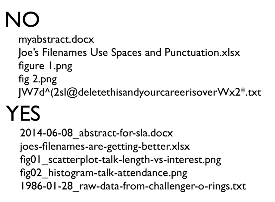
Don’t create multiple versions of the same script (like analysis_FINAL_002_MC.R and analysis_FINALFINAL_003_MC_WM.R.) We’re all familiar with this hellish scenario: you do some work in a Word document (shudder, shudder, the horror, etc.), email it to a colleague, the colleague edits it and sends it back with a tweaked filename, like cool_word_doc_002.docx. Soon enough your hard drive and email client is cluttered with endless iterations of your document. Try to avoid replicating this nightmare in R.
If you do end up with multiple versions, put everything other than the latest version in a subfolder of your “R” folder, called “R/archive”. To avoid a horrible mess of analysis_FINAL_002.R type documents cluttering up your folder, consider using Git for version control.
3.7 Include a README file
Your analysis workflow might seem completely obvious to you. Let’s say that in one script you load raw ABS microdata, run a particular script to clean it up, save the cleaned data somewhere, then load that cleaned data in a second script to produce a summary table, then use a third script to produce a graph based on the summary table. Easy!
Except that might not seem easy or self-explanatory to anyone who comes along and tries to figure out how your analysis works, including you in the future.
Make things easier by including a short text file - called README - in the project folder. This should explain the purpose of the project, the key files, and (if it isn’t clear) the order in which they should be run. If you got the data from somewhere non-obvious, explain that in the README file.
3.8 Keep your workspace clean
Sometimes R doesn’t behave the way you expect it to. You might run a script and find it works fine, then run it again and find it’s producing some strange output. This can be the result of changes in your R environment. You can set different options in R, which can (silently!) affect things. Or maybe you had some different objects - data, functions - defined in your environment the second time round that you didn’t have originally, or some extra packages loaded.
To avoid this situation, keep your workspace tidy. When you load a script, do it in a fresh R session.
But… don’t clean your workspace within your analysis script. People sometimes do this using this command:
This removes all objects from your environment. But it doesn’t completely clear your R environment, and it doesn’t do anything to any packages you have loaded. As Jenny Bryan puts it, this command is “a red flag, because it is indicative of a non-reproducible workflow”.
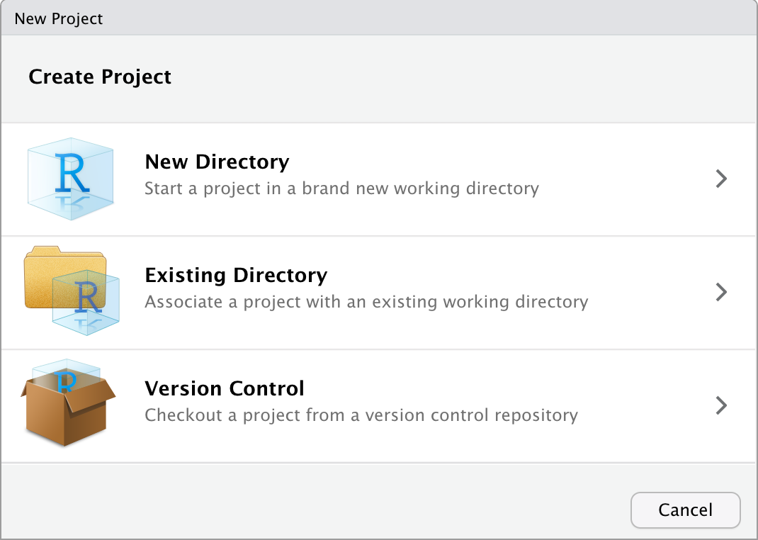
3.9 Quick guide to starting a project
When you’re starting a new project:
- Open RStudio;
- Click ‘File -> New project’
- Click ‘New Directory’
- Click ‘New Project’
- Give your new project a name, choose where it should go, and click ‘Create Project’
- Create subfolders in your project folder using the ‘New Folder’ button (by default in the lower-right pane of RStudio) - start with an ‘R’ folder
- Click ‘File -> New File -> R Script’
- Save your R script in your R folder.
Now you’ve got a good shell of a project - a dedicated folder, with an associated RStudio project, and at least one subfolder. This is a good base to start your work.
Learn more:
- ‘Using RStudio Projects’ by the good people of R Studio
- Danielle Navarro’s wonderful slides on project structures
- Jenny Bryan’s article on project-oriented workflow
- Jenny Bryan’s fantastic presentation on how to name files (it’s fun I promise)